Walk-Through Example: Cell Fate Specification in Ascidian Embryo
In Kobayashi et al., 2018, the authors performed FC analysis from Mochizuki et al., 2013 on a gene regulatory network (GRN) of seven tissues that specifies cell fates in embryos of the ascidian Ciona intestinalis (type A; also called Ciona robusta). After performing FC analysis, the authors identified five key molecules. By controlling the activities of these key molecules, the specific gene expression of six of seven tissues observed in the embryo was successfully reproduced.
In this example, we show how OCSANA+ can reproduce the FC analysis in addition to the results from control experiments in Ascidian embryos. Additionally, we explore how the extended Feedback Vertex Set Control (FC) with source nodes (Zanudo et al., 2017) and OCSANA functionalities could increase the accuracy of simulated results.
For the full results of this example, please see `OCSANA+supplementary file`_
You can download the .sif file used in this tutorial here
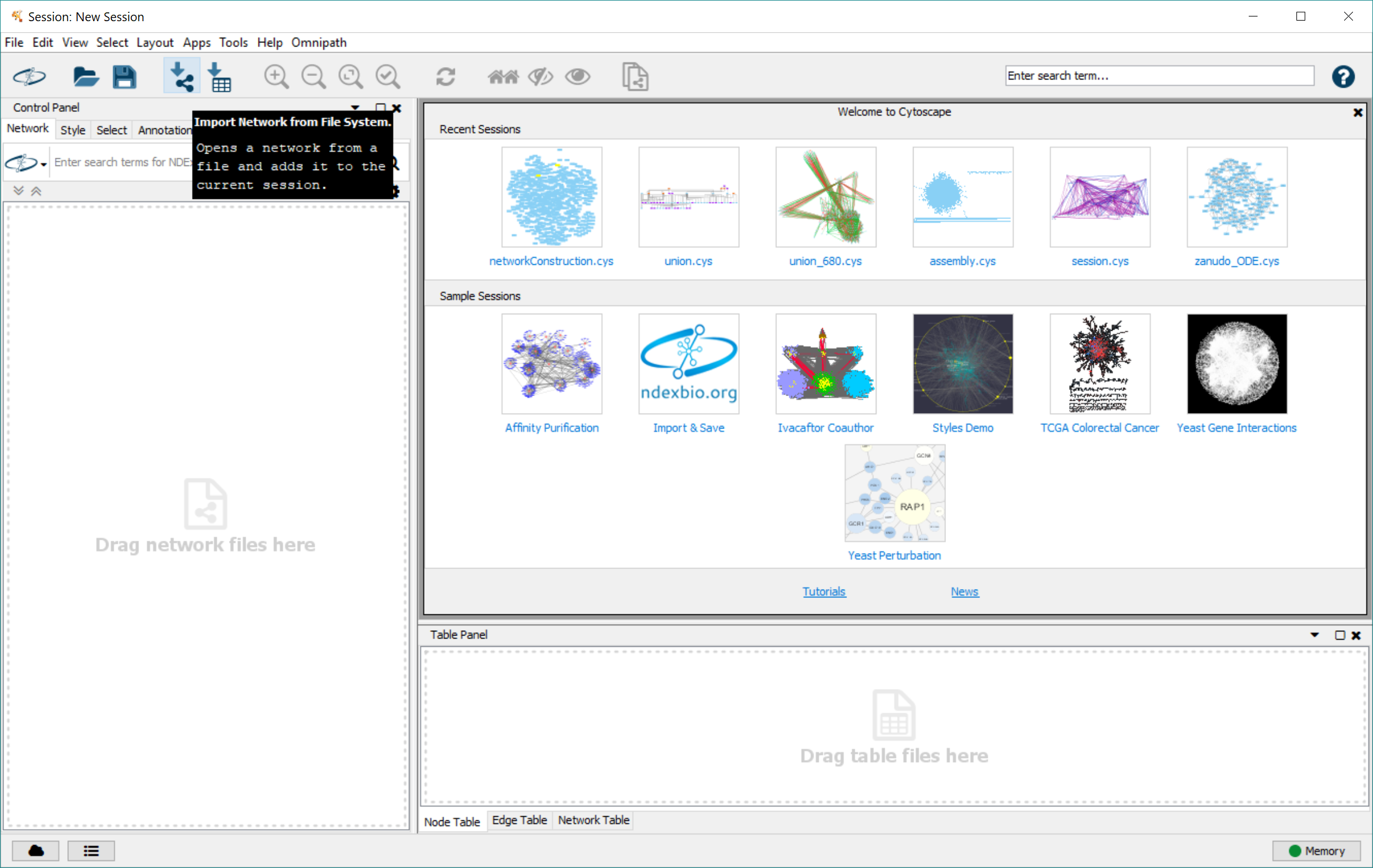
Step 1: Initial Cytoscape Setup
Upon launching Cytoscape, a new session will be opened. You can load the ascidian embryo network by selecting “Import Network from file System” icon in the toolbar
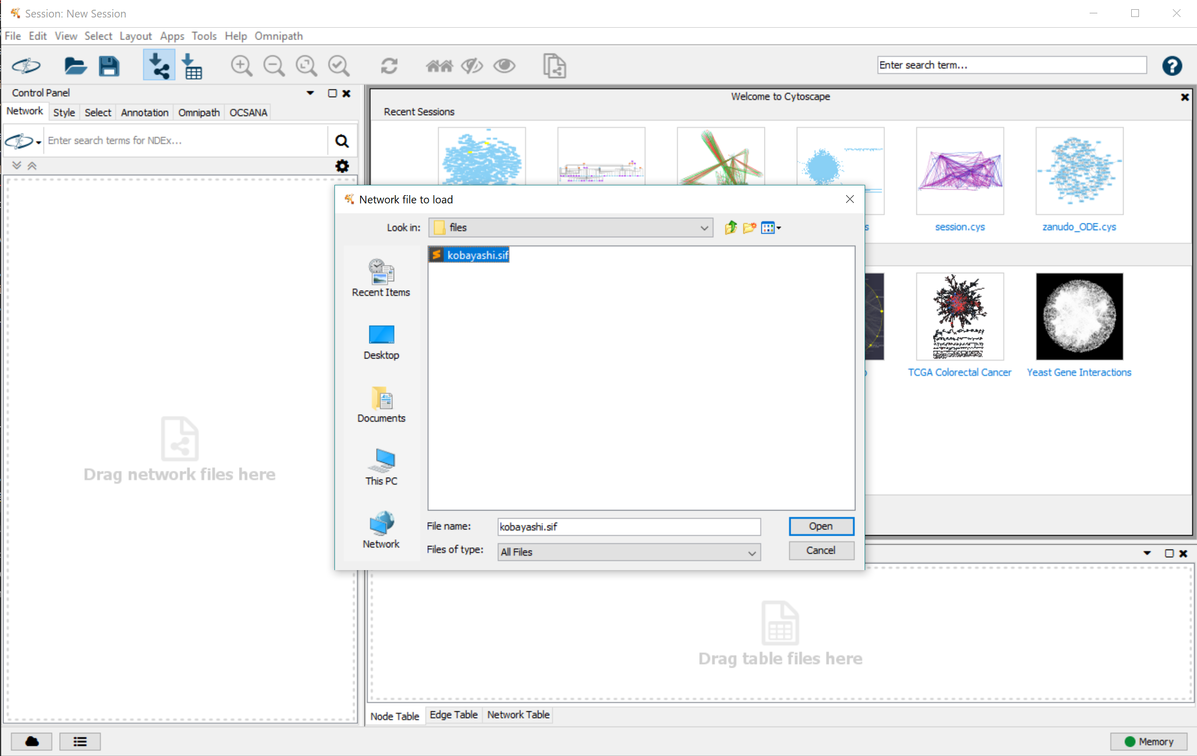
In the pop-up menu, navigate to the folder where you stored the network, and select the file.
Step 2: Identifying Feedback Vertex Set Control Sets (FC)
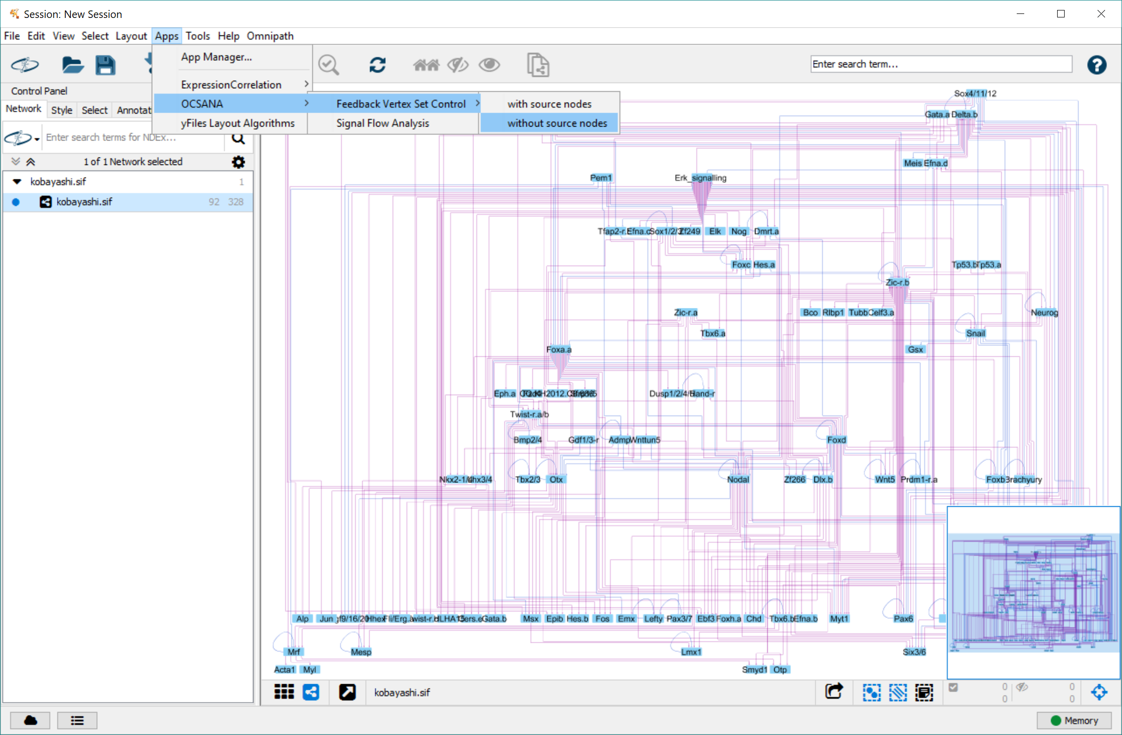
To first reproduce the results of Kobayashi et al., 2018, we perform Feedback Vertex Set Control (FC) Discovery.
From the Apps dropdown in the toolbar navigate to “OCSANA>Feedback Vertex Set Control. OCSANA+ provides two algorithms for identifying FC sets: with or without source nodes (You can read more about these two algorithms in <`OCSANA+ paper supplement`_, Mochizuki et al., 2013, or Zanudo et al., 2017.).
To replicate the results of Kobayashi et al., 2018, select “without source nodes”
In the pop up menu:
- Set “select node name column” to “shared name”
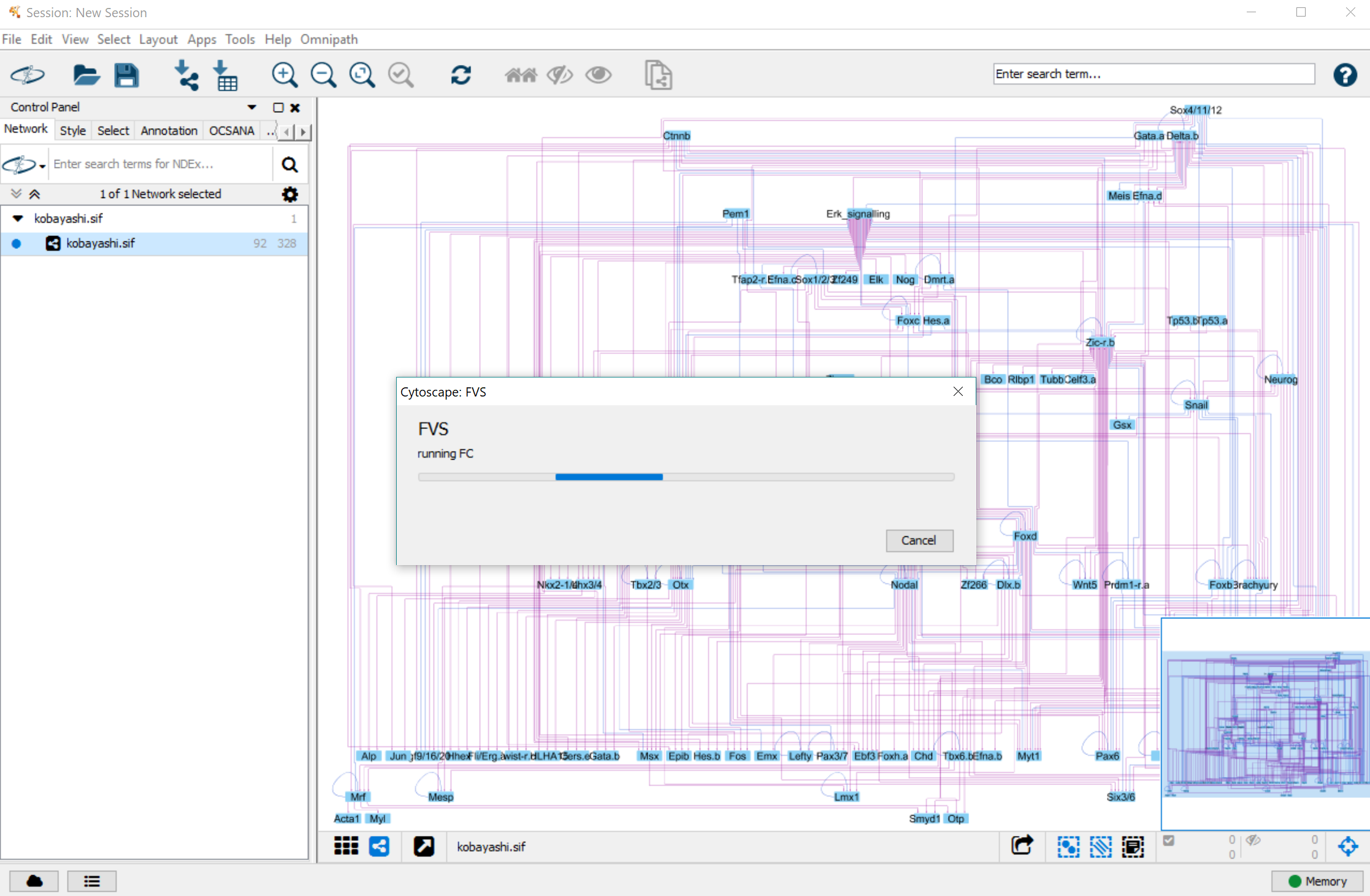
- For this tutorial example, we will do an unbound FVS Discovery search. This will run the FVS algorithm 50 times to identify FVSes. Note that there may not be 50 FVSes in the network, so the number of FVSes returned may be fewer than 50.
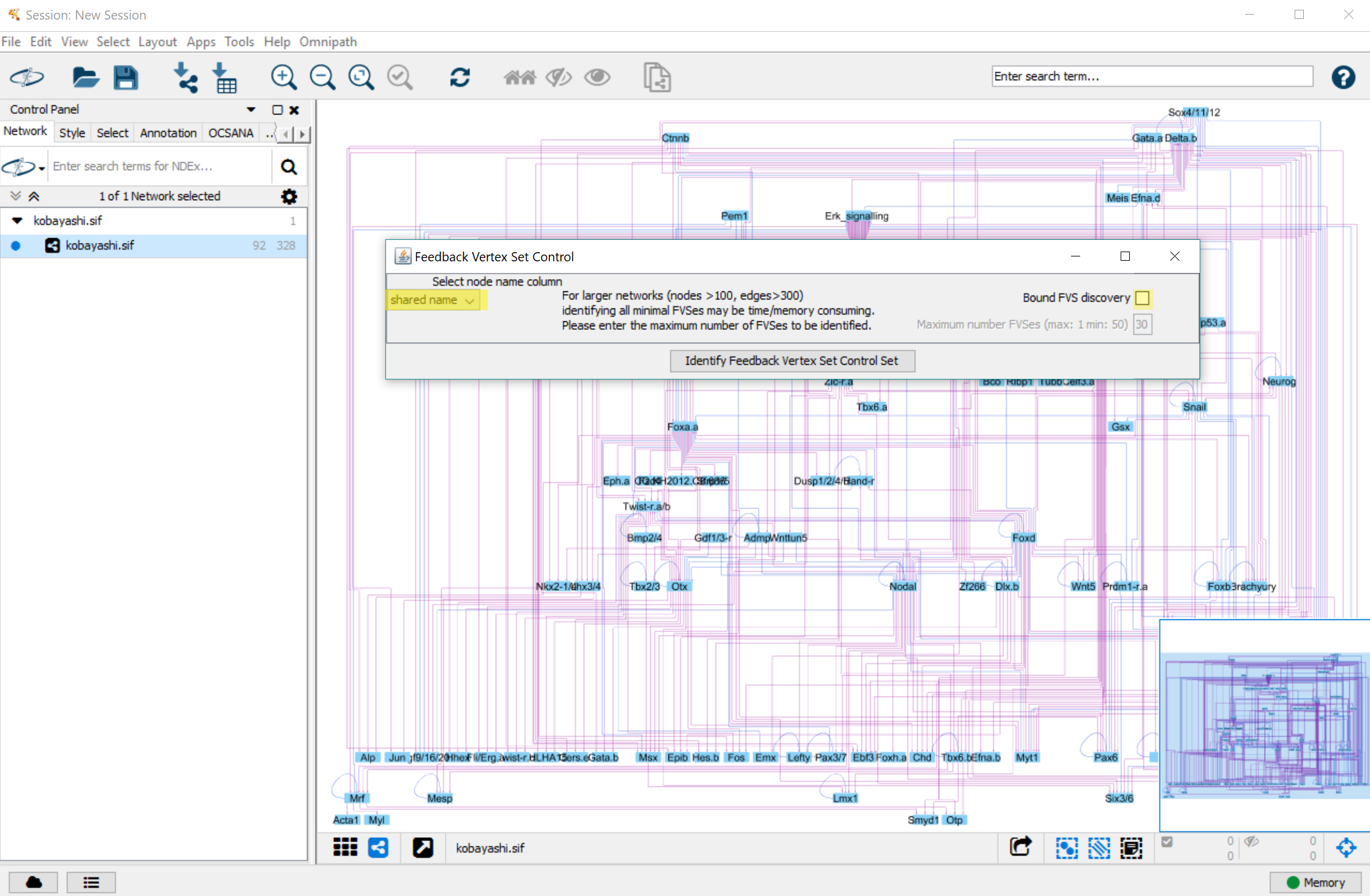
Select “Identify Feedback Vertex Set Control Set”
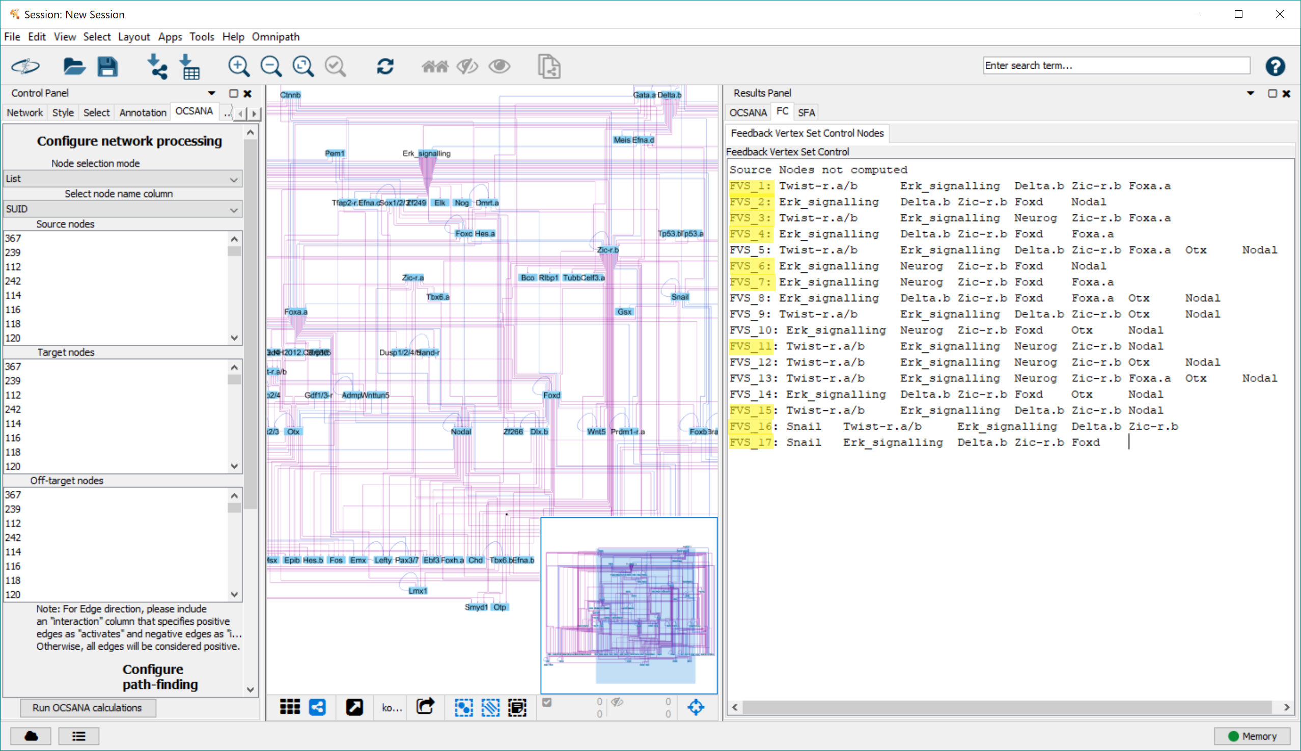
The results will be displayed in the FC subpanel of the Results Panel. Minimal FC sets are highlighted
Step 3: Simulating FC node perturbations using SFA
We will focus on the FC set used in Kobayashi et al., 2018 in vivo perturbations for our simulation with SFA. The FC set consists of the following 5 nodes:
Foxa.a, Foxd, Neurog, Zic-r.b, and Erk signaling
To simulate the experimental results in Kobayashi et al., 2018, we will use Signal Flow Analysis (SFA) to estimate the log steady state values of network nodes (Lee and Cho, 2018)
First, we simulate the “unperturbed” state (no up-regulation or down-regulation of FC nodes), by activation of Gata.a and Zic-r.a which are noted to initiate the zygotic developmental program.
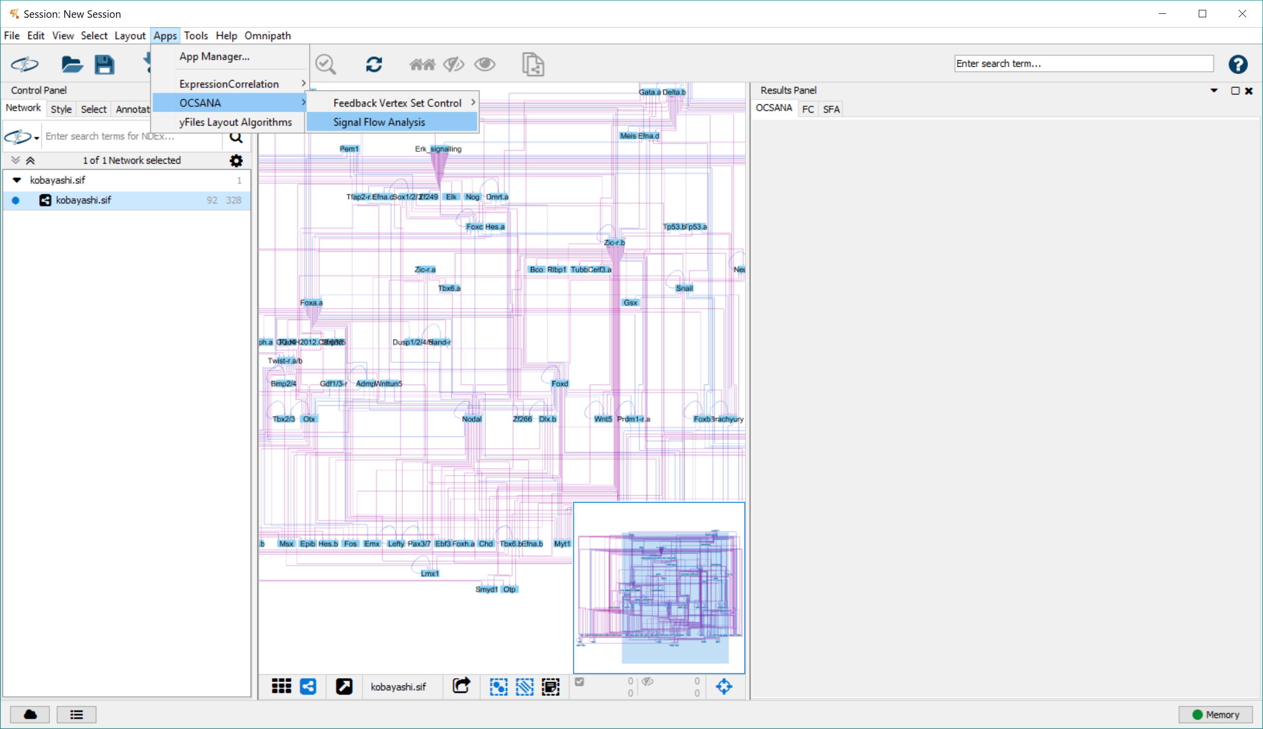
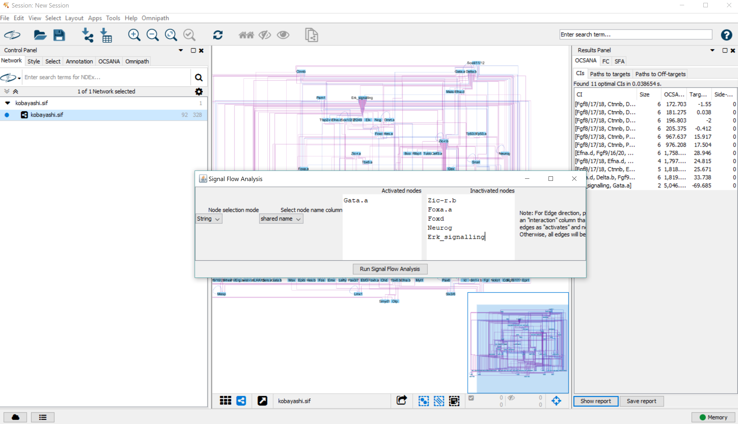
From the Apps dropdown in the toolbar navigate to “OCSANA>Signal Flow Analysis”.
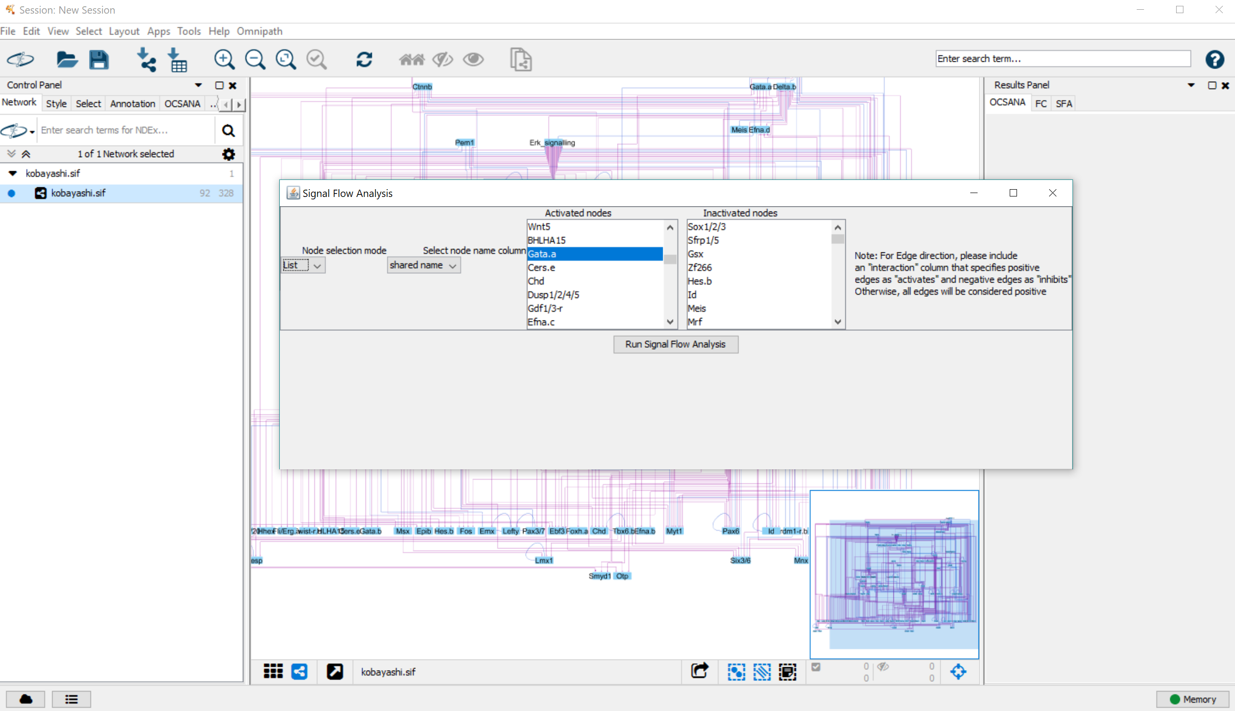
In the pop-up menu:
- select either “List” or “String” for Node Selection Mode
2. select “shared name” for Select Node Name column 3a. If “List” is selected, scroll in the “Activated Nodes” box and ctrl+click Gata.a and Zic-r.a
3b. If “String” is selected, type Gata.a and Zic-r.a into the “Activated Nodes” box (either comma delimited, or newline delimited)
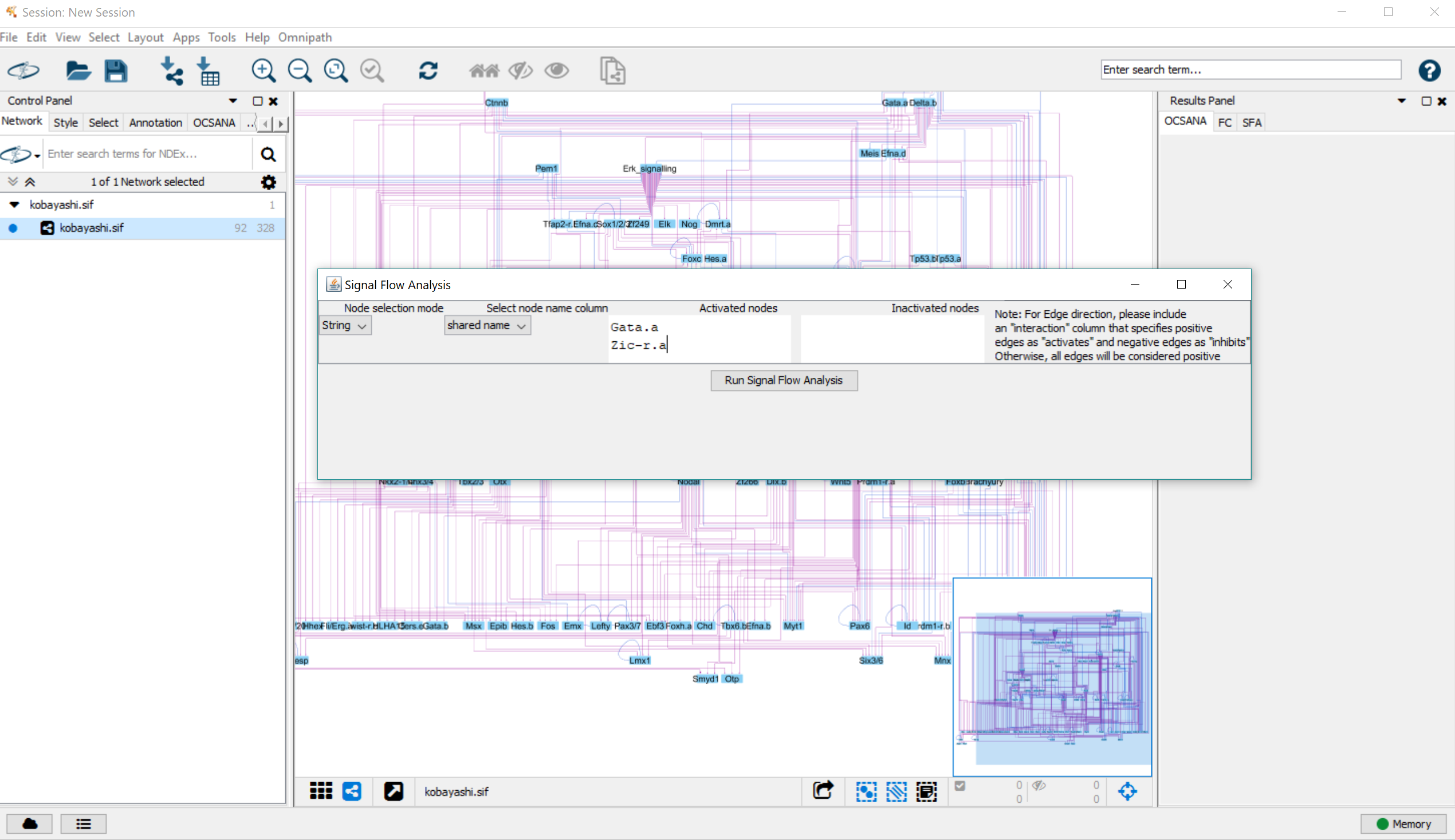
To start SFA, click “Run Signal Flow Analysis”
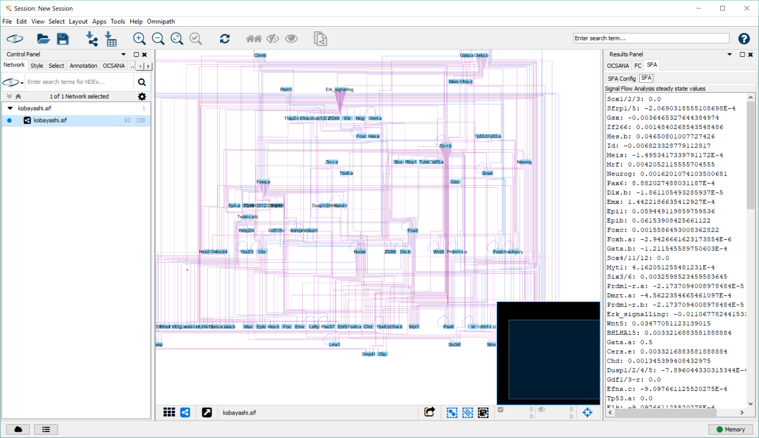
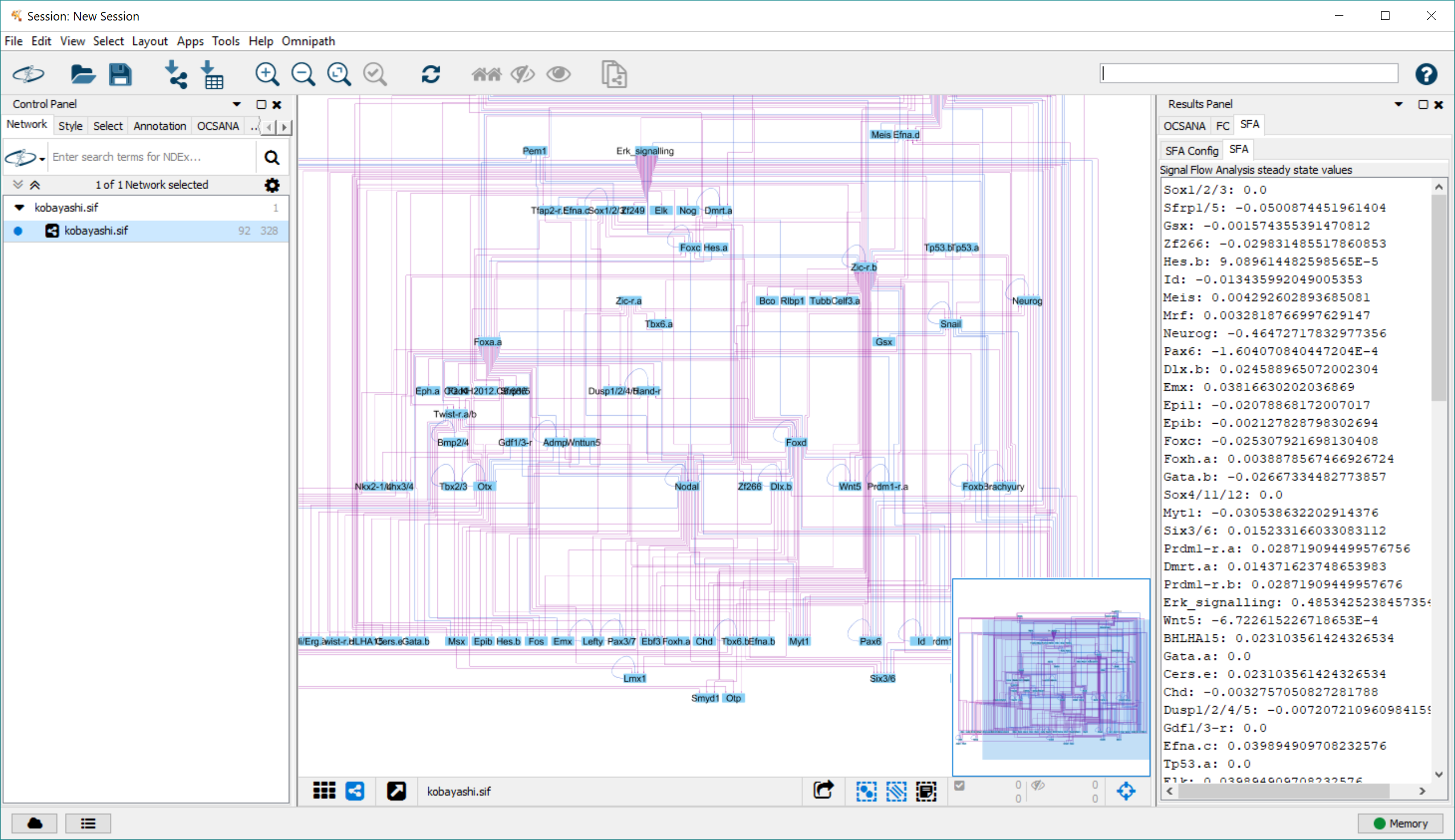
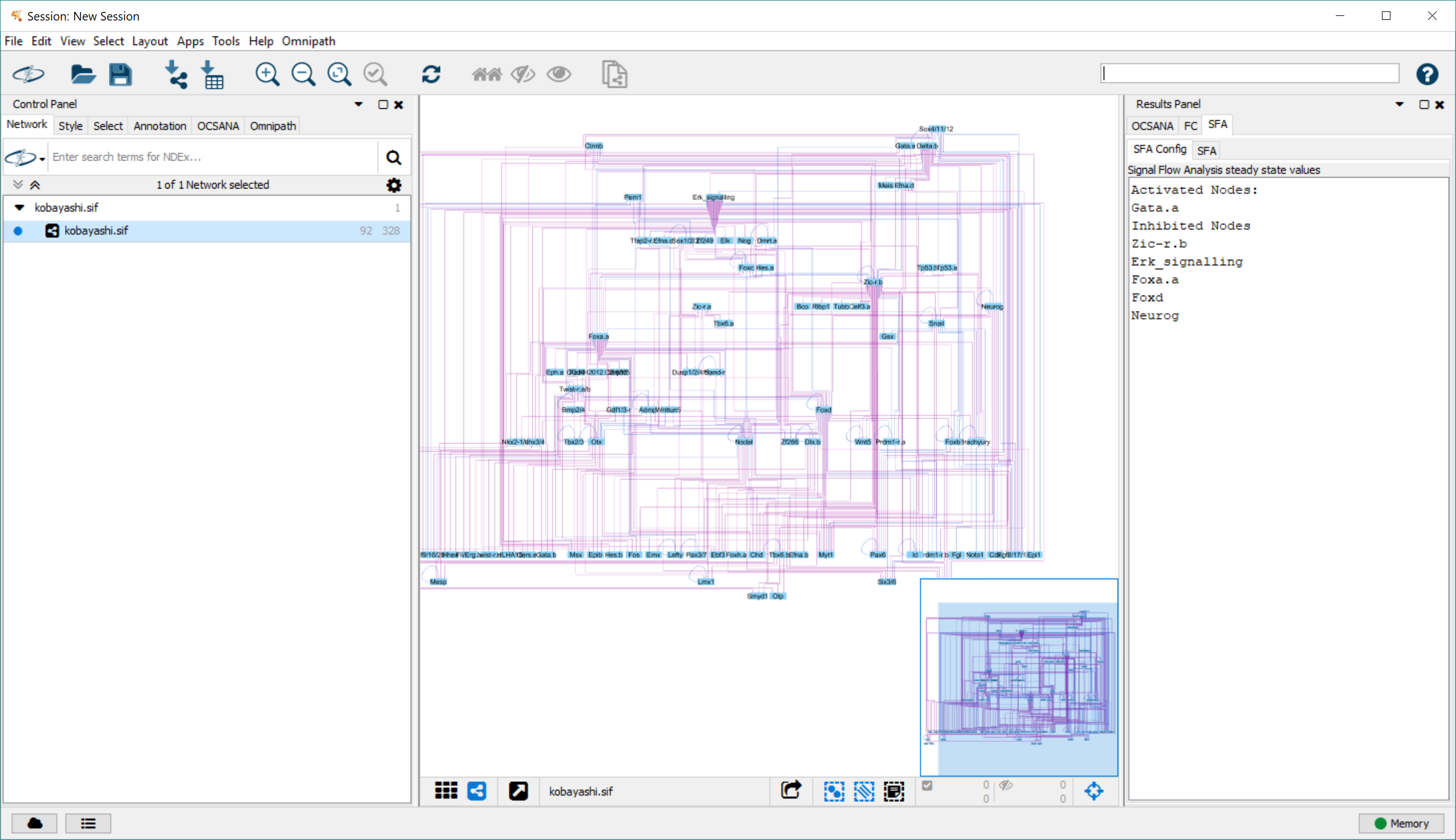
After completion of SFA, the results will appear in the SFA tab of the Results Panel.
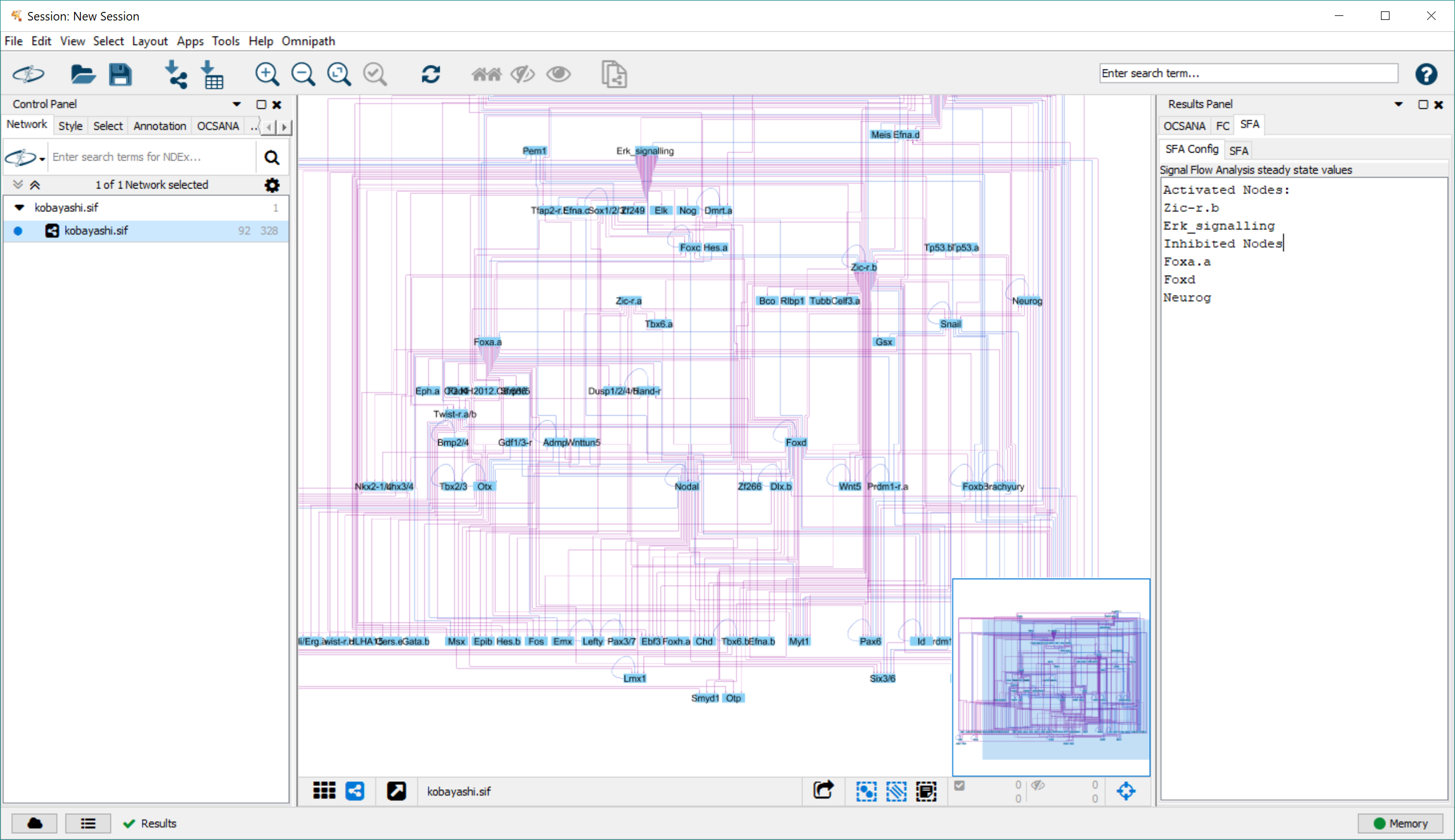
The “SFAConfig” tab displays which nodes were activated or inhibited in the initial user configuration

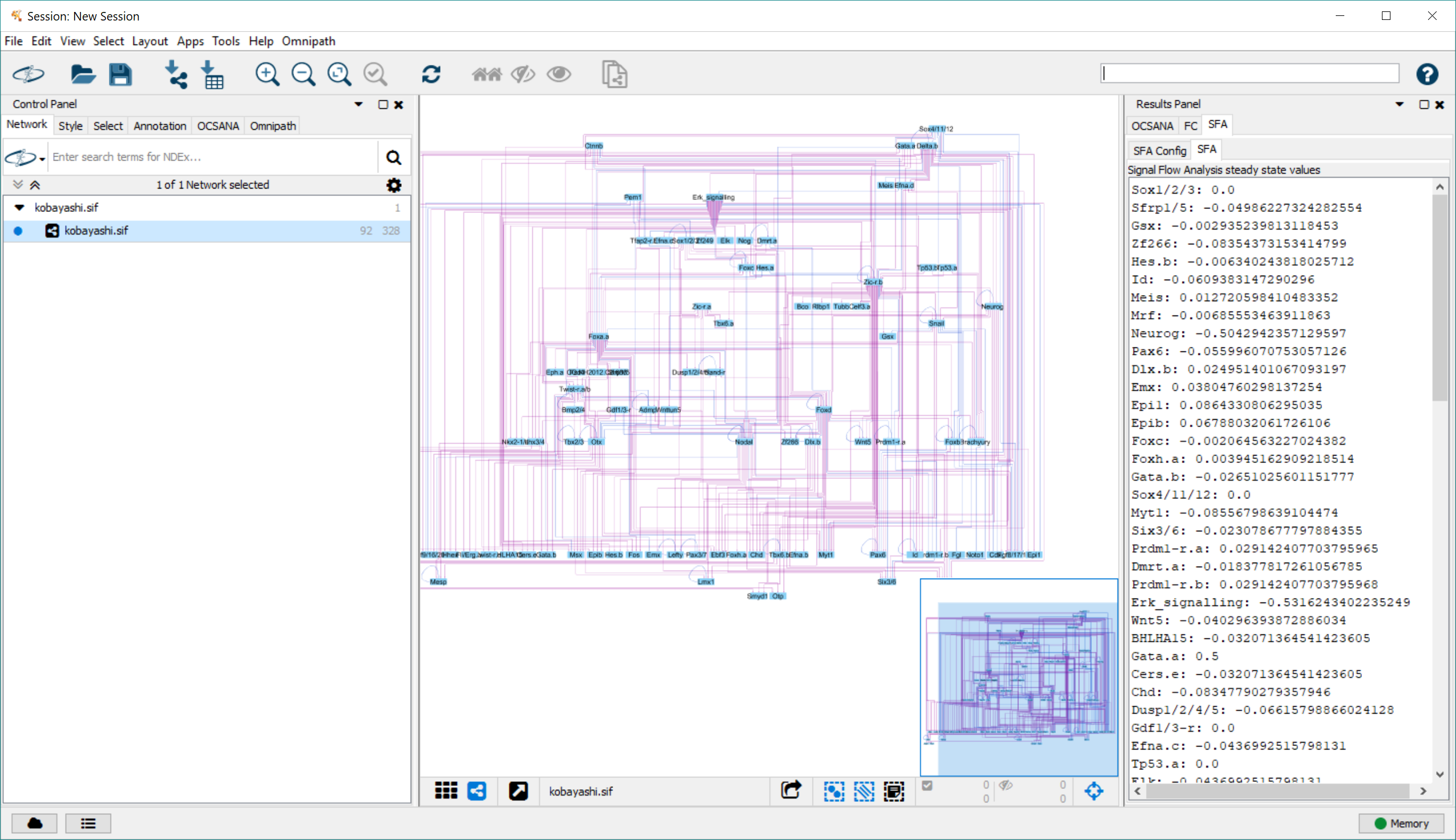
The “SFA” tab displays the steady state log values for all network nodes.
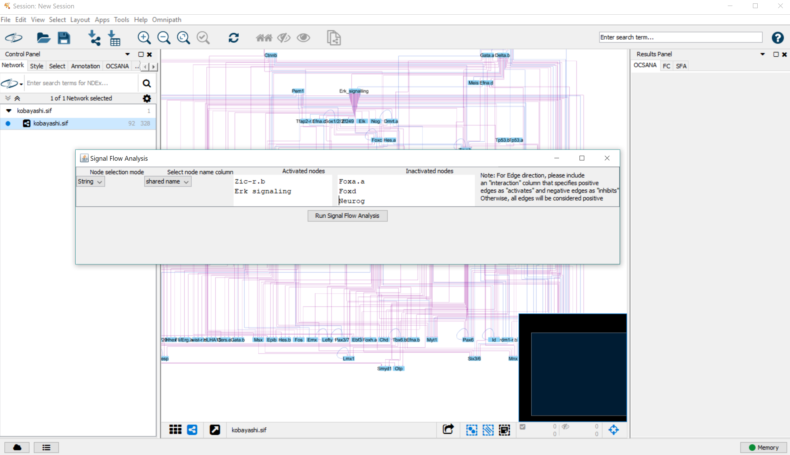
We repeat this analysis performing a perturbation of the FC nodes. For example, as described in Kobayashi et al., 2018, down-regulation of Foxa.a, Foxd, and Neurog and up-regulation of Zic-r.b, and Erk signaling would lead to the mesenchymal tissue cell fate in the ascidian embryo.
We can simulate this experiment using SFA by selecting Zic-r.b and Erk signaling as activated nodes, and Foxa.a, Foxd, and Neurog as inactivated nodes
Again, the configuration and results appear in the Results Panel.
Using the steady state log values produced by SFA, we can calculate a direction of activity change between the perturbed and unperturbed state, synonymous with a logFC value.
For example, the log steady state value produced of mesenchymal marker Fli/Erg.a in the unperturbed state is 0.00332. The value in the above perturbation is 0.02310. by computing the difference of perturbed vs unperturbed (0.02310-0.00332=0.01978), and computing a positive result, we interpret this as Fli/Erg.a upregulated in the perturbed steady state vs unperturbed steady state (to read more about interpreting the output of SFA, see Lee and Cho, 2018).
Let’s check another cell fate marker node. Alp is a marker gene for endoderm specification. The steady state log value of Alp in the unperturbed state is 3.2139E-5. The value steady state log value of Alp in the perturbed state is -0.02999. When we compute the direction of activity change, (-0.02999-3.2139E-5=-0.03002) and receive a negative value, we interpret this as Alp being downregulated under this perturbation.
Identifying Feedback Vertex Set Control Sets (FC) with source nodes
Considering that the GRN studied contains source nodes, which in principle can affect the dynamical attractors in the system, we applied the extended FC approach from Zanudo et al., 2017.
We can use OCSANA+ to compute FC sets with source nodes.
From the Apps dropdown in the toolbar navigate to “OCSANA>Feedback Vertex Set Control>with source nodes”
The pop-up menu is identical to that of step 2.
After setting your configurations and running FC discovery, the FC results subpanel of the Results Panel will display both the FVSes and source nodes
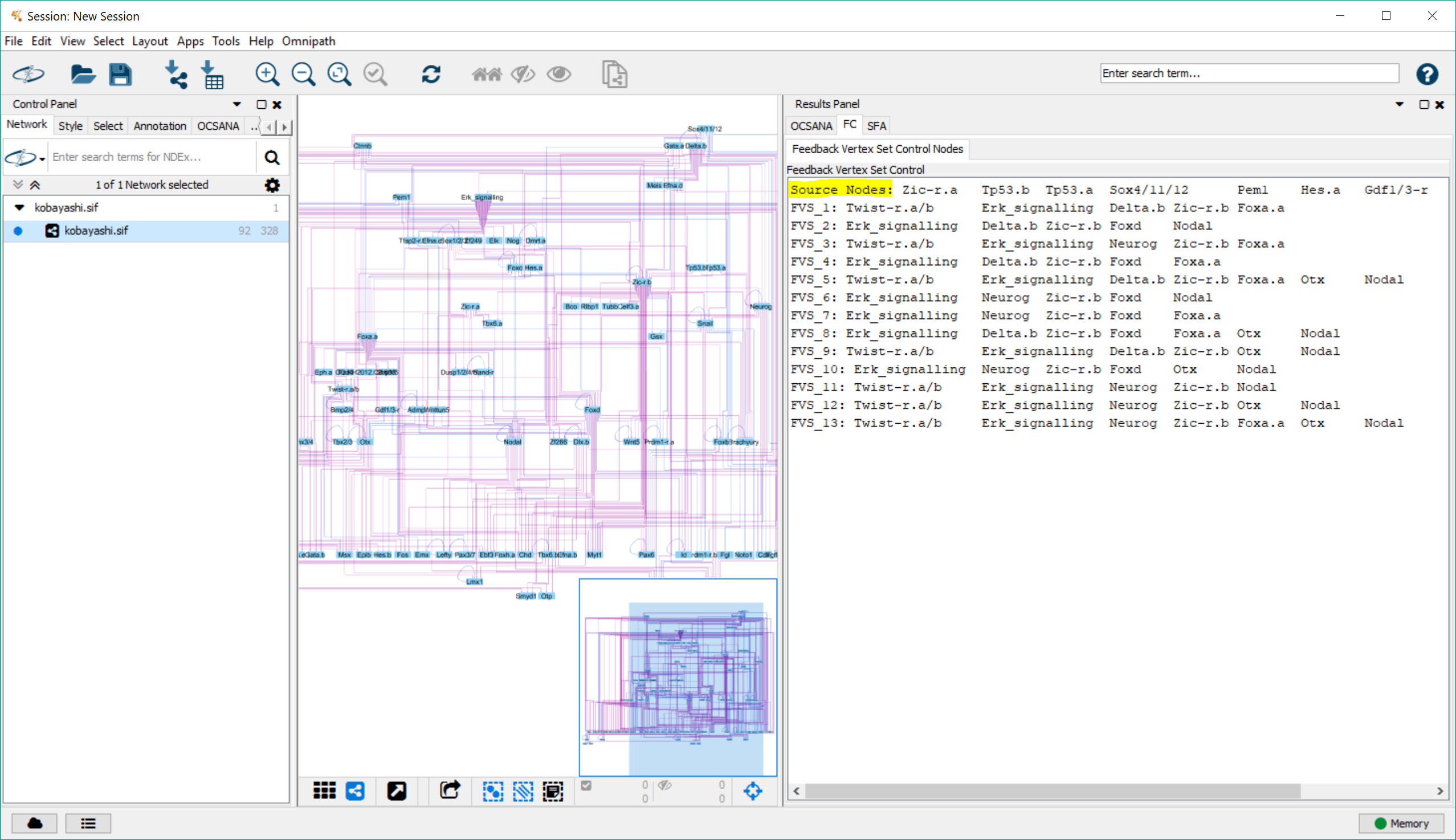
We now have identified the nine source nodes in the network: Ctnnb, Gata.a, Gdf1/3-r, Hes.a, Pem1, Sox4/11/12, Tp53.a,Tp53.b, Zic-r.a
Identifying CIs with OCSANA
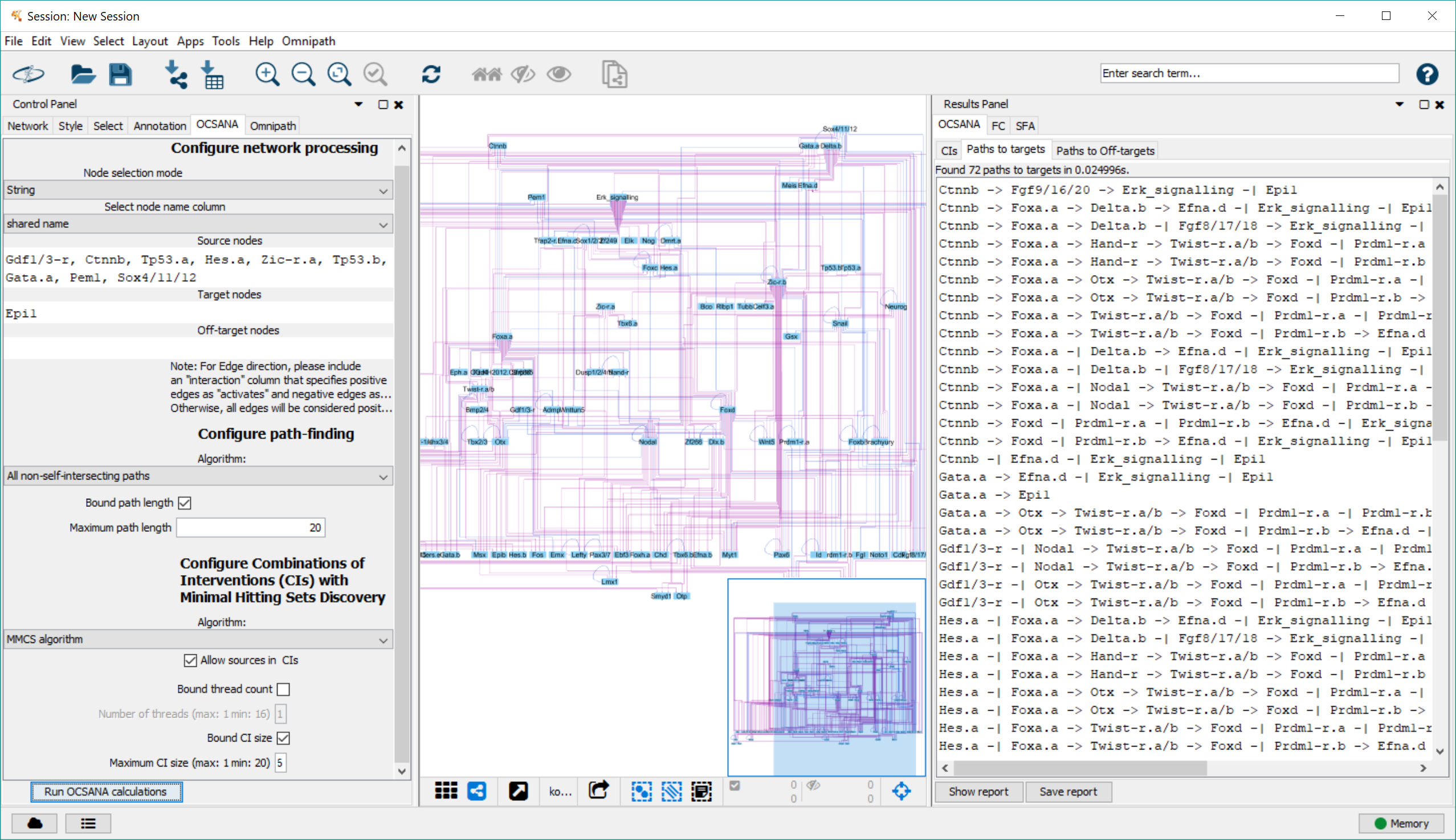
We can use OCSANA in OCSANA+ to canalize the signal from the network source nodes to a specified cell fate. For example, if we want to predict additional nodes that may control the signal to epidermal specification, we identify combinations of interventions that can be used to intervene in paths from the nine source nodes to epidermis marker Epi1.
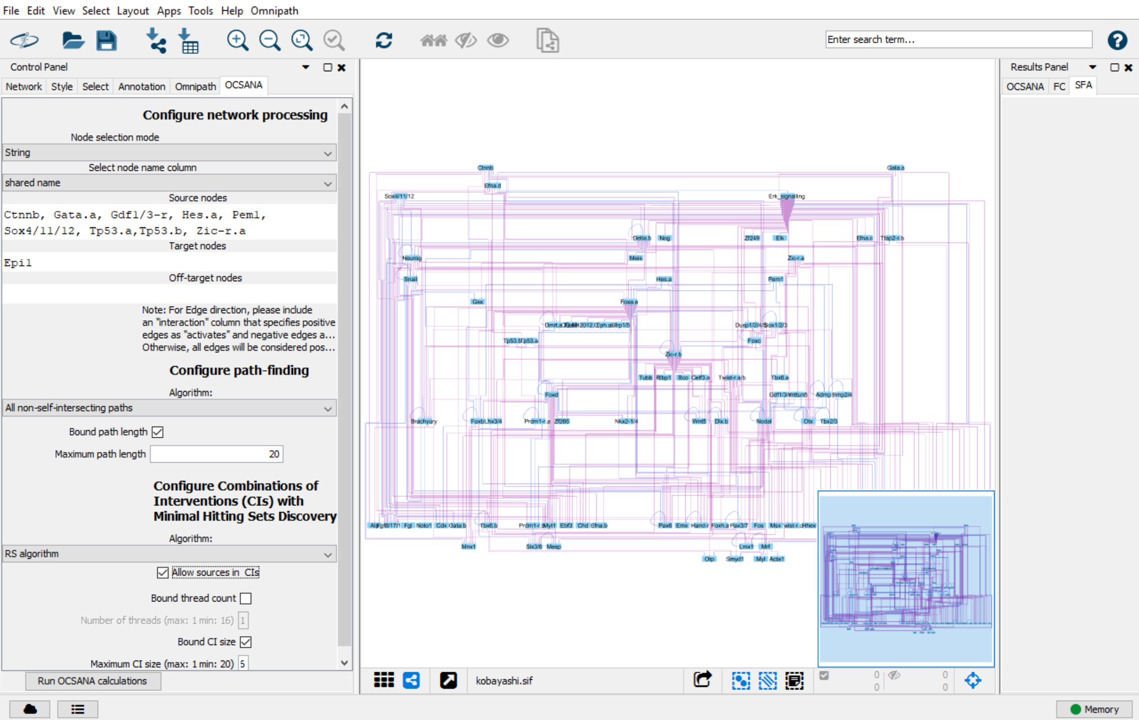
In the OCSANA panel in the Cytoscape Control Panel:
- select either “List” or “String” for Node Selection Mode
- select “shared name” for Select Node Name column
- Enter the nine source nodes in the source nodes box
- Enter Epi1 in the target nodes box
- We have set to discover all non-self intersecting paths with a length limit of 20 nodes from source to target. This setting can be changed to suit your network needs and size
- To configure CI discovery we have chosen the RS algorithm. We will check “allow sources in CIs” so that source nodes can be considered in CIs. We will not bind the number of threads. We will bind CI size at 6 nodes.
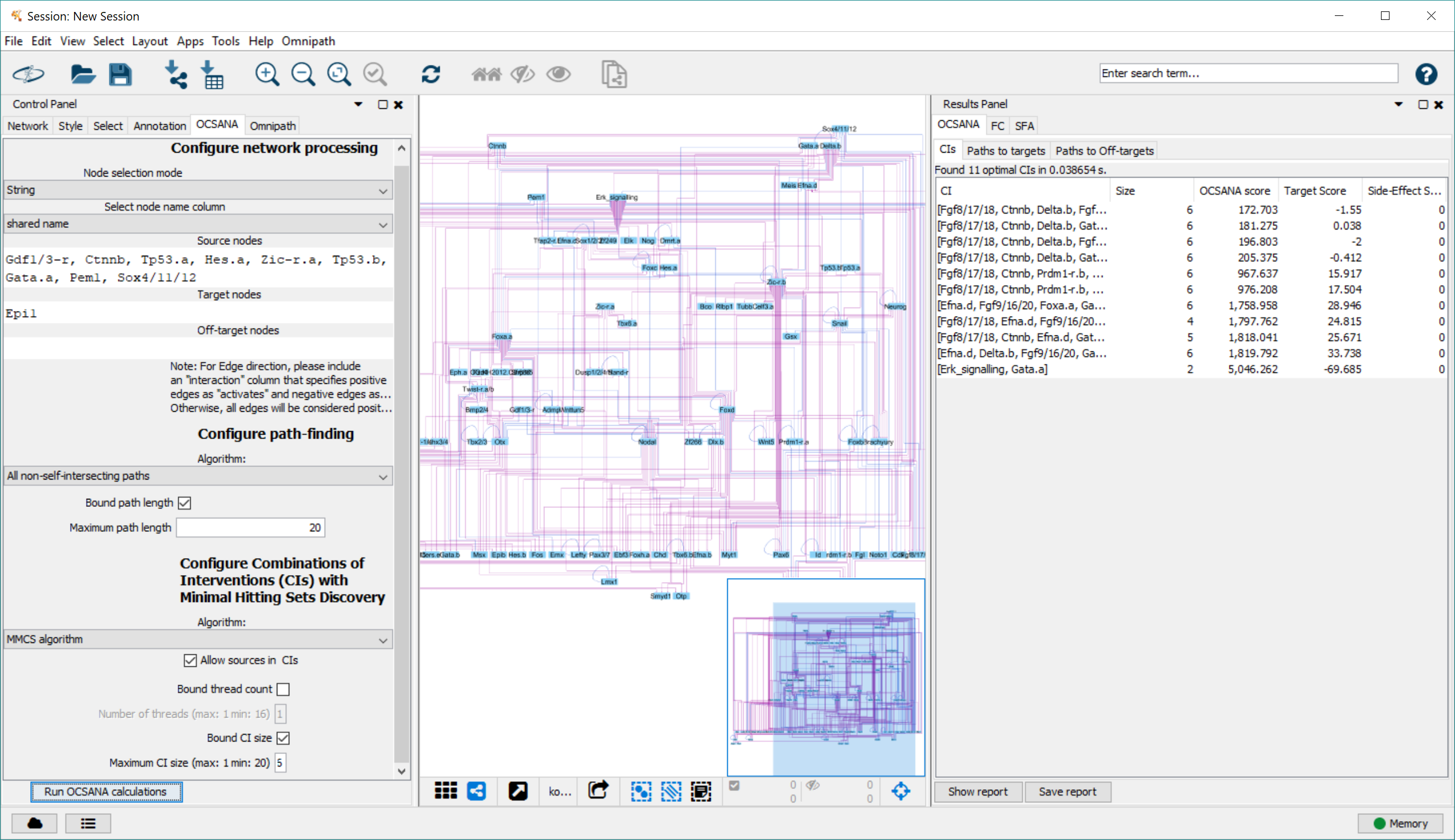
After configuration, click “Run OCSANA analysis”
Once the OCSANA Run has completed, the results will appear in the OCSANA Subpanel of the results panel.
The CI tab displays the minimal CIs discovered under user settings
The paths to targets tab displays the paths from the nine source nodes to Epi1
Simulating FC and CI node perturbations using SFA
We will choose the smallest CI of 2 nodes (Gata.a and Erk signalling) to use in combination with the FC perturbation specified in Kobayashi et al., 2018 (down regulation of FC nodes) to simulate the results for epidermal tissue specification. Do note that Erk signalling is a node within the FC set.
Using SFA, we will set the activated nodes to Gata.a and inactivated nodes as Foxa.a, Foxd, Neurog, Zic-r.b, and Erk signalling
After running SFA, we see the results in the results panel
Again, we can calculate the logFC between the above perturbation and the unperturbed steady state for Epi1 (0.08643-0.05944=0.02699). We see that the value is positive; therefore Epi1 is upregulated in the perturbed steady state when compared to the unperturbed steady state.